Source Datasets Used
NOAA Sea Level Rise Data – NOAA has developed sea level rise GIS layers (raster and polygon options) that represent current sea levels, and potential flooding from one to six feet of sea level rise for all coastal US states and territories except Alaska. Sea levels represent the mean higher high water level, which is a long-term average of the highest high tide that occurs in a day (many locations experience two high tides and two low tides each day). The methods used to map sea level rise inundation are described by the NOAA Office for Coastal Management (NOAA 2017, entire).
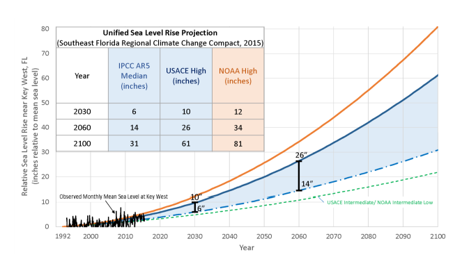
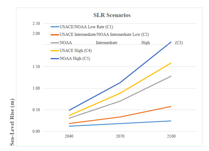
To estimate loss of habitat due to inundation from sea level rise for coastal populations of Eastern indigo snakes, we used NOAA’s shapefiles available at their online sea level rise viewer (NOAA 2018). Projected sea level rise scenarios from NOAA provide a range of inundation levels from low to extreme. We chose the most likely scenario based on the Sea-Level Rise Working Group (SLRWG 2015), which corresponds to NOAA’s intermediate-high scenario. Local scenarios are available at 29 locations along the coast of Florida, with each scenario providing estimates of sea level rise at decadal time steps out the year 2100. We found the average sea rise level estimate for the intermediate high NOAA scenario across all 29 stations and used this estimate to project habitat loss at 2050 (2 feet sea level rise) and 2070 (3 feet sea level rise). Loss of habitat due to sea level rise was in addition to loss of habitat due to urban development.
https://coast.noaa.gov/digitalcoast/tools/slr.html
SLEUTH Urbanization Data – We used the Slope, Land cover, Exclusion, Urbanization, Transportation, and Hillshade (SLEUTH; Jantz et al. 2010, entire) model to determine areas predicted to be urbanized in the future. The SLEUTH model has previously been used to predict probabilities of urbanization across the southeastern US in 10-year increments, and the resulting GIS data are freely available (Belyea and Terrando 2013, entire). For our future projections, we used the SLEUTH raster data sets from the years 2050 and 2070, and examined the area predicted to be urbanized with 20%, 50%, or 90% probability depending on the scenario.
We considered using the FL2070 (citation) urbanization model that was developed specifically for Florida, but comparisons of the FL2070 and SLEUTH baseline (current) urbanization models revealed that the SLEUTH model was more accurate in identifying current urbanization in moderately to highly developed areas than the FL2070 model (which was more accurate than SLEUTH in low density developed areas).
Eastern Indigo Snake Rangewide Potential Habitat Model – We calculated habitat area using the habitat model described in Appendix C, which identifies and ranks suitable habitat.
Projecting Resilience Factors
We used the above datasets to generate future predictions for population extent, population connectivity, habitat quantity, habitat type, and urbanization under three urbanization scenarios (high, moderate, and low urbanization) at two time points, 2050 and 2070. The 2050 time point was associated with one predicted foot of sea level rise, and the 2070 time point was associated with a prediction of two feet of sea level rise. The following summarizes each population and habitat factor (Table D1)
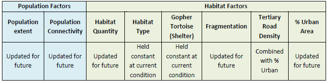
1. Population Extent – Measured as the cumulative of area of each population created by overlapping 5-mile (8 km) buffers of the eastern indigo snake records, as it was measured in the current condition. The only time population extent changed between current to future conditions for any population was when land area within the current population extent was predicted to be inundated by sea level rise in the future. In these instances, the future population extent was equal to the current population extent minus the area of land predicted to be inundated.
2. Population Connectivity – Measured as the overlap and presence of connected suitable habitat among populations within a 5-mile buffer around populations. This “population connectivity buffer,” is represented by a 10-mile buffer around eastern indigo snake records (or 5-mile buffer from record = population plus an additional 5-mile buffer to assess overlap (i.e. connectivity) among populations.
We measured this habitat factor the same way as we did for current condition but used the updated potential habitat layer with losses from urbanization and sea level rise for each scenario. We counted the number of overlapping “population connectivity buffers” for each population. Then we examined the habitat (Easter Indigo Snake Habitat Model, Appendix C) within the overlapping area. Populations were considered “connected” if habitat patches were present between populations and were not bisected by one or more primary or secondary roads. Resilience categories were defined as: High: population connected to 2 or more populations, Medium: population connected to at least 1 other population, Low: population connectivity buffer overlaps with at least one other population connectivity buffer but is fragmented by major road (primary or secondary). Very Low: population is not connected to another population. See Figure B2, Appendix B for illustration.
3. Habitat Quantity and Type – Habitat quantity (acres) of habitat for each habitat type (primary, secondary and tertiary), and in total, was calculated for each population using the Eastern Indigo Snake Habitat Model (Appendix C), with habitat removed for predicted future sea level rise and urbanization. Habitat was removed by overlaying sea level rise (one foot for 2050, two feet for 2070) and predicted urbanization (20%, 50%, and 90% for high, moderate, and low urbanization scenarios, respectively, in both 2050 and 2070) onto current habitat in GIS. Habitat that overlapped with the increased sea level or predicted urbanization was removed from the calculation of future habitat quantity. We did not predict changes in habitat type (primary, secondary, or tertiary) habitat in the future due to high amounts of uncertainty in how land use will change.
4. Gopher Tortoise (Shelter) – Held constant as current condition. Appendix B for more detail.
5. Habitat Fragmentation – Using the Eastern Indigo Snake Habitat Model (Appendix C), fragmentation was assessed by re-calculating the area of habitat patches of different sizes for each population for each scenario. Habitat patches for this assessment could contain all three types of habitat (primary, secondary and tertiary). Breaks in habitat patches reflect significant breaks in habitat connectivity or non-habitat between patches and often were due to primary or secondary roads, major water bodies and other areas of non-habitat. Additional information on habitat fragmentation metrics can be found in Appendix C.
6. Tertiary Roads and % Area Urbanized – Percent of urbanized area was calculated for each population using the 2050 and 2070 outputs of the SLEUTH model. The SLEUTH model provides a probability that each pixel (60 x 60 m) will be urbanized. We assessed urbanization in 2050 and 2070 at three urbanization probabilities. A 20% or more probability of being developed is very inclusive and represented a high development scenario. A 50% or more probability of being developed included only those pixels that were more likely to be developed than not, and represented a medium development scenario. A 90% or more probability of development is the most restrictive scenario we assessed, where only pixels that are very likely to be developed were considered, representing a low development scenario.
Weights assigned to factors in Table D1.
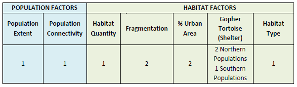
Habitat factors were given the same importance weights as applied to the current condition analysis, except tertiary road density was combined into percent urban area in the future scenario analysis (Table D2). It is difficult to predict how tertiary roads will change in the future (e.g. tertiary roads becoming primary or secondary roads and where new tertiary roads will occur). Tertiary road density and percent urban area are highly correlated (Appendix B, Figure B3) therefore we combined these two factors and their weights into one, therefore percent urban was given a weight 2 for both northern and southern populations.
See Appendix B for additional rational for weighting habitat factors.
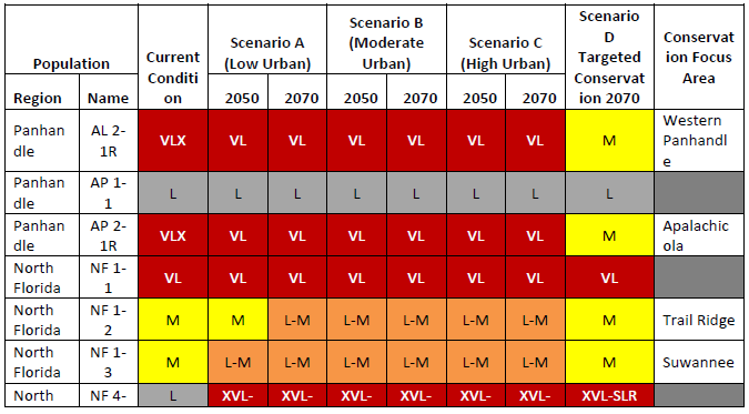
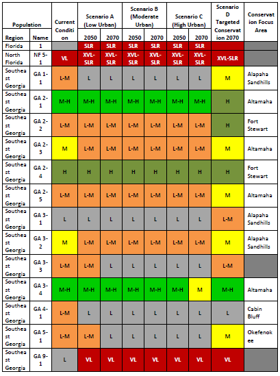
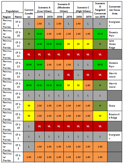
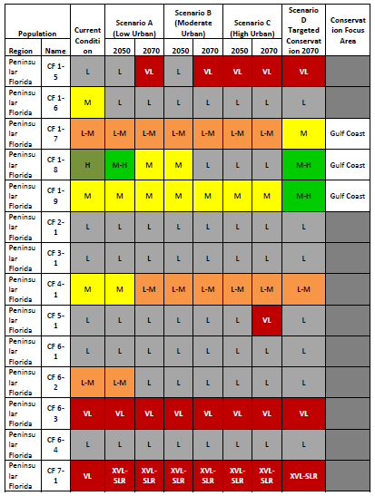
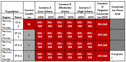
H= High; M-H= Medium-High; M= Medium; L-M= Medium-Low; L= Low; VL= Very Low; XVL-SLR are those populations extirpated due to sea level rise. AL2-1R* and AP2-1R* are repatriation sites. Therefore, overall condition for these two sites is considered Very Low or Extirpated (VLX). There are 30 extirpated populations shown in Figure 21 in section 5.1 of the report that are not included in this table.
References
Belyea, C. M. and A. J. Terrando. 2013. Urban growth modeling for the SAMBI Designing Sustainable Landscapes Project. North Carolina State University. http://www.basic.ncsu.edu/dsl/urb.html. Accessed 10 March 2018.
Jantz, C. A., S. J. Goetz, D. Donato and P. Claggett. 2010. Designing and Implementing a Regional Urban Modeling System Using the SLEUTH Cellular Urban Model. Computers, Environment and Urban Systems 34:1-16.
NOAA Office for Coastal Management. 2017. Method description: Detailed method for mapping sea level rise inundation. 5 pp. https://coast.noaa.gov/data/digitalcoast/pdf/slr-inundation-methods.pdf, Accessed 8/15/2018.
Sea-Level Rise Working Group (SLRWG). 2015. Unified sea level rise projection: southeast Florida. A Document Prepared for the Southeast Florida Regional Climate Change Compact Steering Committee, 35 pp.